

2 Stochastic Factor of Safety Analysis of Slope in Clay
The following example considers the determination of the factor of safety for the slope shown in Figure 2.1. The material is Tresca and the undrained shear strength is modeled as a random field with a mean value of 70 kPa and a coefficient of variation of 30%. The vertical and horizontal correlation lengths are 2 m and 50 m respectively. These values of COV and correlation lengths correspond roughly to those indicated by Phoon and Kulhawy (1999) as being characteristic for undrained shear strength.
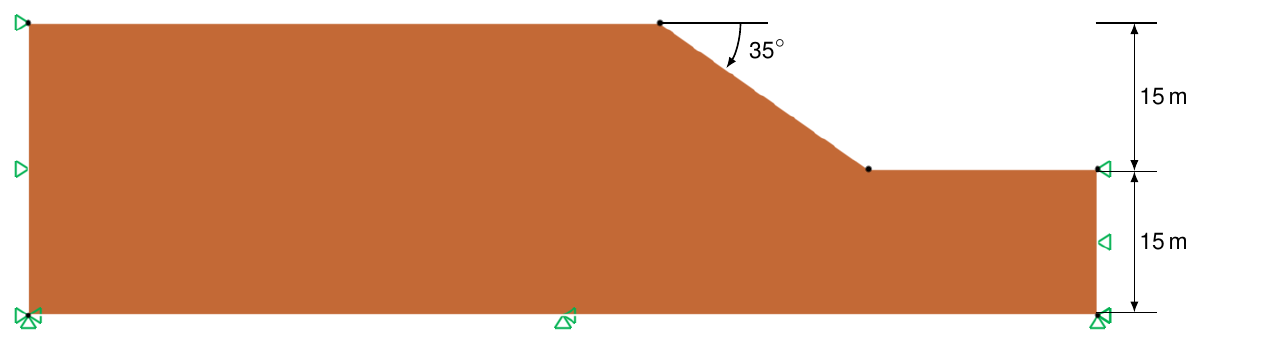
Figure 2.1: Slope in clay with random undrained shear strength.
Before the actual stochastic analysis proceeds, a standard deterministic analysis with s_u = 70 kPa is conducted to be used later for comparison purposes. The result of this analysis is a factor of safety given by
\text{FS} = 1.45 \tag{2.1}The collapse mechanism is shown in Figure 2.2.
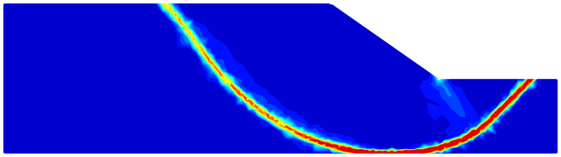
Figure 2.2: Collapse mechanism for deterministic analysis with constant s_u = 70 kPa.
As in the previous example, the factor of safety is determined by means of Limit Analysis (now with Multiplier = Gravity) using 1,000 upper and lower bound elements with 3 adaptivity iterations. The factors of safety reported in the following are the mean values between each upper and lower bound run. A total of 1,000 Monte Carlo runs are conducted.
The results in terms of probability distributions of the factor of safety are shown in Figure 2.3. Also shown are the distributions corresponding to infinite correlation lengths (mean value = 1.45 and standard deviation = 1.45 \times \text{COV}/100\% = 0.435). Since the characteristic length scale of the failure mechanism is much larger than the vertical correlation length, the COV of the resulting factor of safety (11.4%) is significantly smaller than the inherent COV of the undrained shear strength (30%). The mean value is also somewhat smaller (1.31 vs 1.45) while the probability of failure is much less (1.0% vs 13.2%). These results follow the same trend as those of the previous example for a footing width much larger than the vertical correlation length.
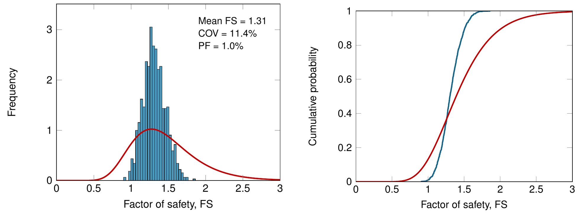
Figure 2.3: Probability functions for factor of safety. The red curves correspond to infinite correlation lengths.
The probability distribution of mobilized mass is shown in Figure 2.4. We see that the distribution tends to be somewhat bimodal with a peak around 600 m³/m and another one around 1,400 m³/m. These two values represent two distinct families of failure mechanisms, the latter being deeper than the former. Examples are shown in Figure 2.5.
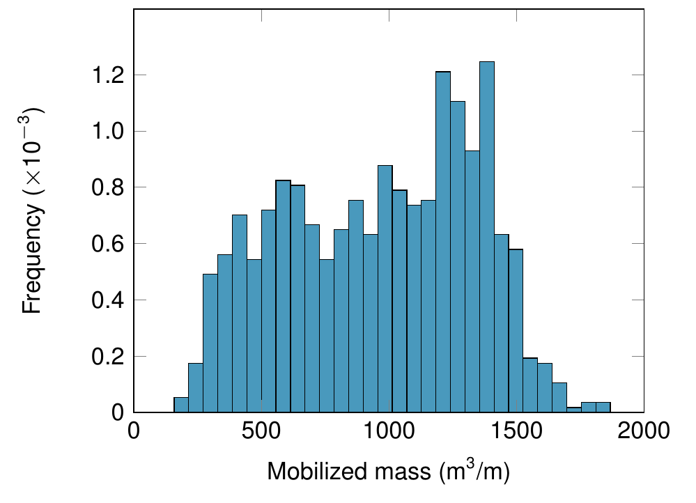
Figure 2.4: Probability distribution of mobilized mass.
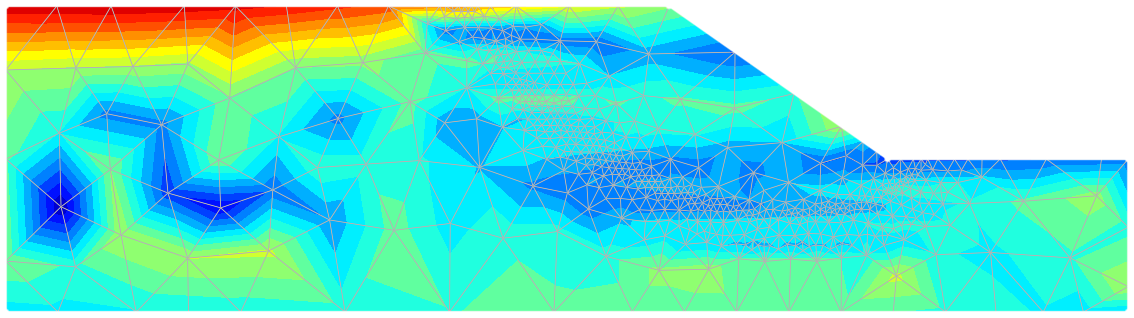
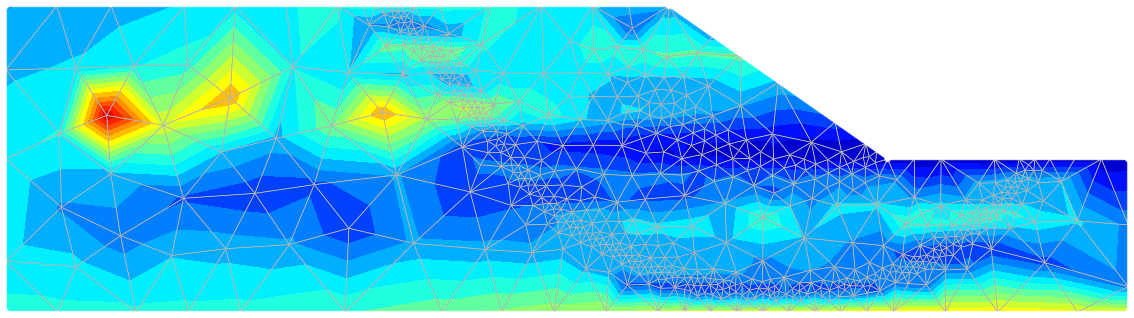
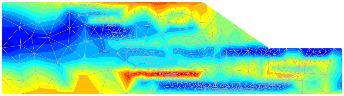
Figure 2.5: Examples of shallow (a), intermediate (b) and deep (c) failure mechanisms. From top to bottom: (a) run no 569, mobilized mass = 601 m³/m; (b) run no 599, mobilized mass = 1,001 m³/m; (c) run no 366, mobilized mass = 1,400 m³/m.
Code
"""Preample"""
from OptumGX import *
gx = GX()

"""Project setup"""
project_name="Stochastic slope in clay"
project = gx.create_project(project_name)
model = project.get_model('Model A')
model.name = 'Clay slope'

"""Constants"""
cu = 70

"""Model Setup"""
model.add_polygon([[35,15], [-30,15], [-30,-15], [80,-15], [80,0], [56.42,0], [35,15]])

shapes = model.select([0, -0.001], types='face')
material = project.get_material('Tresca Basic')
material.cu = cu
solid = model.set_solid(shapes, material)

model.set_standard_fixities()

model.zoom_all()

"""Analysis and output"""
model.set_analysis_properties(
    analysis_type= 'factor_of_safety',
    # load_multiplier_multiplier = 'gravity',
    mesh_adaptivity= 'yes',
    adaptivity_iterations=3)

project.run_analysis()

print('Factor of safety: ', model.output.critical_results.factor_of_safety)

current_path = os.getcwd()
filename =project_name+".gxx"
gx.save_project(file_path=os.path.join(current_path, filename))