# Python Scripting with Spyder

1. Download and install the Spyder IDE from the official website: https://www.spyder-ide.org/download
2. Close Spyder before taking the next steps.

This section contains the necessary steps to prepare a Python working environment using Optum's Python Interpreter and Python Virtual Environment.

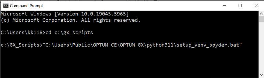
1. Create an empty folder for your GX Python scripts. For example C:\GX_Scripts. All Python scripts are to be placed in this folder (or in folders within the folder, e.g. C:\GX_Scripts\Project 1, C:\GX_Scripts\Project 2, and so on).
2. Open a Windows Command Prompt in the empty folder created and run the following command to setup an environment: C:\Users\Public\OPTUM CE\OPTUM GX\python311\setup_venv_spyder.bat

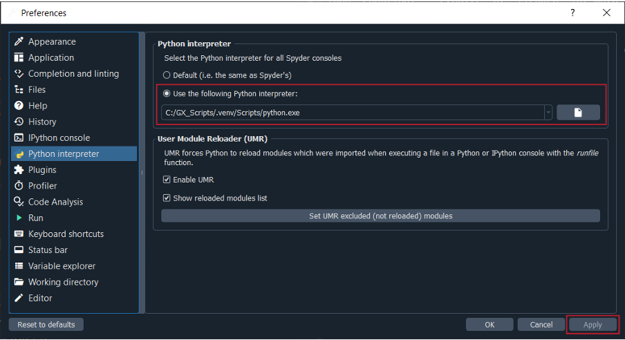
This will create a .venv folder inside the GX scripts folder. This should never be deleted or modified manually.

3. Open Spyder. Under Tools/Preferences/Python Interpreter, change the Python interpreter to the interpreter inside the created .venv folder. For example, with the above created folder, C:\GX_Scripts\.venv\Scripts\python.exe. Apply and close the Preferences dialog.

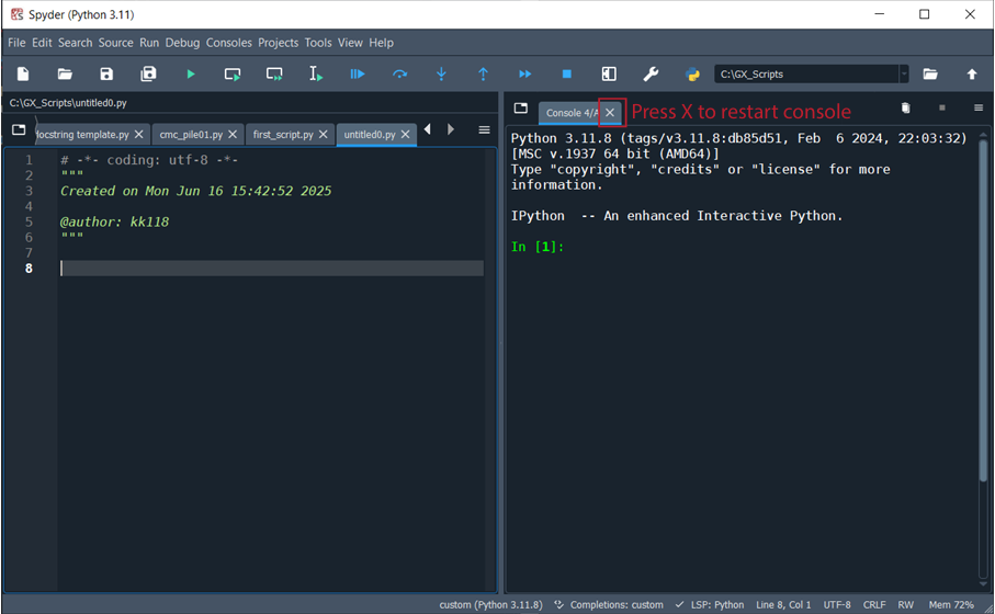
4. Restart the console.

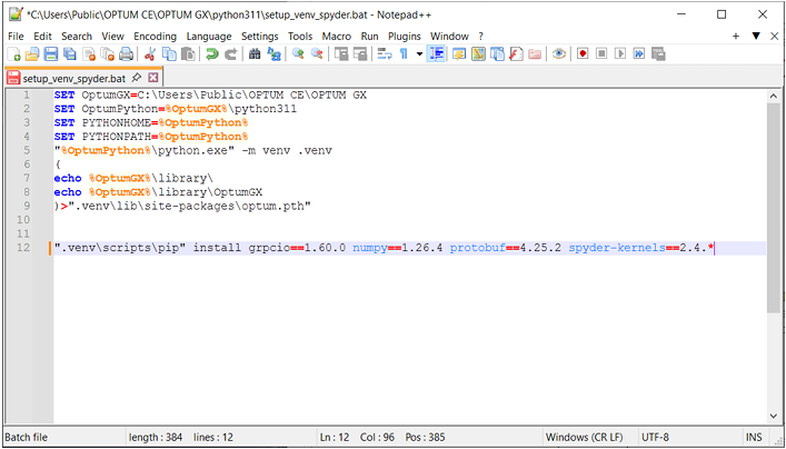
Step 3 of the above installs the so-called Spyder kernels needed for Spyder v. 6.0.7. For other versions of Spyder, different kernels may be needed. Therefore, when restarting the Spyder console (step 4 above), you may encounter a message of the kind:

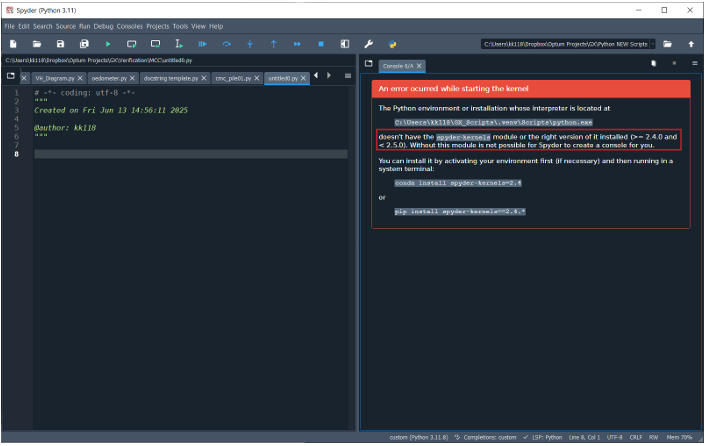
This indicates that the incorrect Spyder kernel has been installed. In the above case, what is needed is version 2.4. This is fixed by editing the file:

C:\Users\Public\OPTUM CE\OPTUM GX\python311\setup_venv_spyder.bat.

Change the default spyder-kernels==3.0. to spyder-kernels==2.4. (or appropriate version as revealed when restarting the Spyder console).

Finally, close Spyder and repeat steps 2-4 above.

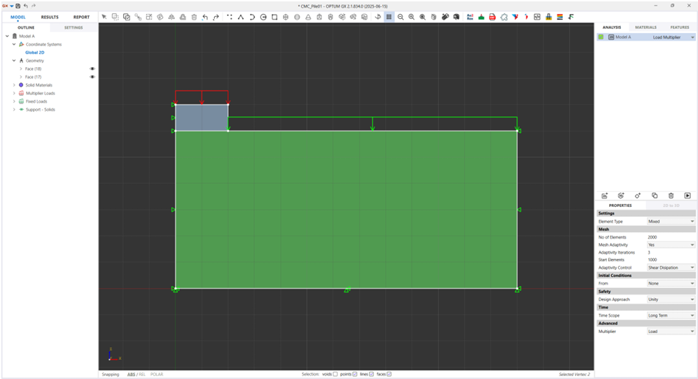
You should now be up and running and can use Spyder for GX scripting. The script shown below calculates the foundation capacity for the problem shown in Figure 3.1.

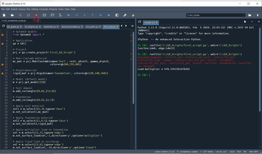
The full code is listed below.

# OptumGX module
from OptumGX import *

# Application
gx = GX()

# Project
prj = gx.create_project('First_GX_Script')

# Mohr-Coulomb material
mc_mat = prj.MohrCoulomb(name='Soil', c=10, phi=25, gamma_dry=18,
color=rgb(80,155,80))

# Rigid material
rigid_mat = prj.Rigid(name='Foundation', color=rgb(120,140,160))

# Model (default model)
m = prj.get_model()[0]

# Soil domain
m.add_rectangle([0,0],[13,6])

# Foundation
m.add_rectangle([0,6],[2,7])

# Apply soil material
sel = m.select([5,3],types='face')
m.set_solid(sel,mc_mat)

# Apply foundation material
sel = m.select([1,6.5],types='face')
m.set_solid(sel,rigid_mat)

# Apply multiplier load to foundation
sel = m.select([1,7],types='edge')
m.set_surface_load(sel,-1,direction='y',option='multiplier')

# Apply fixed load as surcharge
sel = m.select([3,6],types='edge')
m.set_surface_load(sel,-10,direction='y',option='fixed')

# Standard fixities & zoom all
m.set_standard_fixities()
8
FIRST SCRIPT
m.zoom_all()

# Analysis settings
m.set_analysis_properties(analysis_type='load_multiplier',
element_type='mixed',
no_of_elements=2000,
mesh_adaptivity=True,
start_elements=1000,
adaptivity_iterations=3)

# Run analysis
prj.run_analysis()

# Extract and display load multiplier
LM = m.output.global_results.load_multiplier
print('Load multiplier = '+str(LM))